If there are two things that you need to sort out in your incoming data before it hits your OLAP database, they are:

1. Nested data
2. Differently shaped incoming data

Many of the data sources I care most about suffer from both.

Nested data

Why do we have so much nested data?

Both data sources and storage systems have been made to effectively use (and at times prefer) nested data (usually nested JSON).

1. APIs and Microservices have JSON as the lingua franca
2. Streaming schemas also being nested first, carrying their event payloads with embedded context
3. Document stores and NoSQL dbs allowing for this, at scale, pretty easily

Nesting is elegant: it reduces repetition, keeps context close, and evolves easily without migrations.

In OLAP, columnar engines thrive on predictable, typed columns and low-cardinality filters. Nested JSON breaks that rhythm, unless you reshape it first. Throwing a high cardinality JSON column in the middle, without any special treatment, negates many of the benefits of OLAP (though it still can be more efficient than other architectures).

This is a hard problem to deal with, but there are easy ETL and “in database” patterns for dealing with this static nestedness.

But even if you flatten every nested field, you’re still not safe — many pipelines also send rows that don’t share the same shape at all.

Differently shaped data

To me, the more elusive problem is differently shaped incoming data.

Variably nested JSON

Consider the JSON objects:

A buyer on their laptop buys a water bottle, and a bag of chips.

This is a super rational application of data nestedness and flexible schemas, where the ability to have multiple line items reduces:

1. The amount of rows on a flattened database
2. The complexity of the schema in a relational model

In a flattened schema, you’d have to create two rows (one for each line item), repeating all the other fields (and having a bunch of nulls for the irrelevant metadata fields, the performance implications of which we’ll chat about in a later article).

If you have a classic relational model, with here, a couple fact tables transaction and line_item_details, and a dimension table for customers, you’ll have to join all those tables to make any sense of how many customers bought water bottles, which is fine in this toy, but not at 100 million rows (or even a million rows).

Variable Logs

It is not just JSON that suffers from these very efficient, but difficult for OLAP patterns.

I was probably hit hardest by this in my career looking at telemetry, log and metric data in the form of pipe delimited logs, where each log line might be in a different structure. If you’re lucky, there’s a key or event code you can use to look up a schema. But again, this can vary on each row.

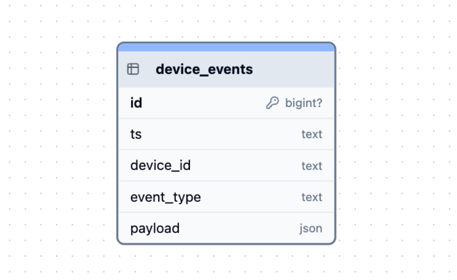
Consider this toy example

Here, we have a key column:

• 1001 → a metrics record containing event_type, timestamp, device_id, cpu, mem, disk
• 1002 → an event record containing event_type, timestamp, device_id, event, reason, uptime

Each row shares the same context columns (timestamp, device_id) but diverges in its payload structure, illustrating how a single log stream can mix multiple event shapes under one roof: efficient for ingestion, painful for OLAP.

Why is this done though? This is pretty efficient, and can be smashed into a telemetry lake. And specialist telemetry services (hi Splunk, hi Datadog, hi Sysdig 👋) will happily parse the data at query time.

Downsides to this in OLAP

As we’ve discussed, both of these structures are rational. And they both fit their purpose.

But we aren’t talking about the purpose they were collected for. We are in the analytical world. In OLAP. Columnar OLAP engines thrive on predictable, typed columns and low-cardinality filters. Drop a high-cardinality JSON blob in the middle and you lose most of that magic, unless you reshape it first.

So the efficiency gains these nested, variable data patterns offer upstream come at a cost: they shift complexity and compute downstream.

Again, this is OK if you are trying to pinpoint a single event in its context to understand why one switch went down 45 minutes ago. But if you are trying to run analytics over time, this is extremely costly (in time, compute and money).

How OLTP deals with this (briefly) and why this doesn’t work for OLAP

In OLTP use-cases, I’ve generally seen two approaches:

1. “Abusing” flexible columns: using string or JSON columns, often decorated with a timestamp to at least make the data somewhat filterable. (Note, even JSON typed rows usually break index use).
2. Normalizing by shape: using more sophisticated data processing to pare out records into a set of tables whose schemas reflect each data type, related via foreign keys (e.g. a few fact and dimension tables, congruent with OLTP design principles).

The common approach of abusing a poor payload field

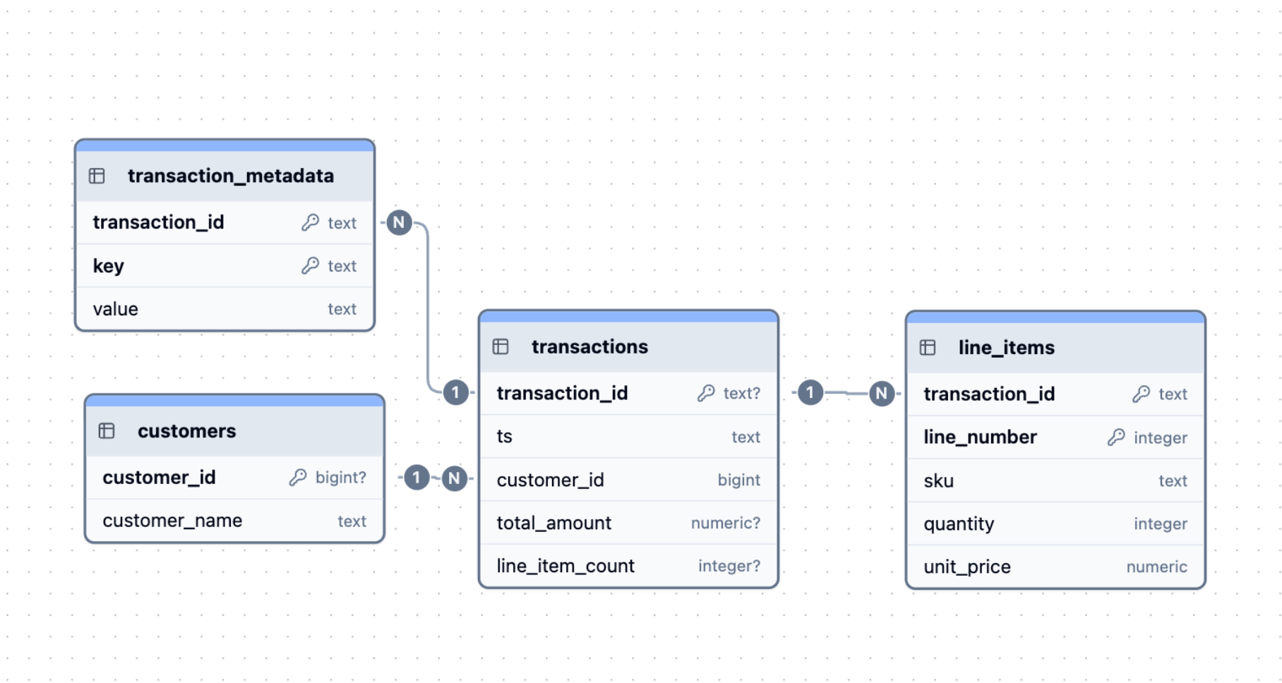An example of the use of a relational model for storage, efficient, but requires multiple joins to reconstruct the log.

Both of these options are somewhat acceptable in OLTP databases and OLTP query paradigms, since the use-case usually involves finding some tiny subset of transactions and extracting them for analysis. As long as the key filterable fields (like timestamp, device_id, even event_type) are extracted and indexed, the database can locate that subset efficiently.

The heavy lifting (parsing the JSON blob or the log row, or joining multiple tables to “rehydrate” a record) happens on just a few rows. Which is absolutely fine for OLTP query patterns.

In OLAP, though, the same approach becomes disastrous.

Scanning millions of rows with embedded JSON or performing rehydrating joins at scale destroys the performance benefits of a columnar engine — and turns every query into a CPU-bound parsing job.

Patterns for dealing with this in OLAP

Like every other article in this series, I’ll start by reiterating: OLAP is read-optimizated and columnar. It also relies on types and data similarity to allow for its accelerated processing using SIMD (Single Instruction Multiple Data, which we spoke about yesterday, only works when the same simple instruction is applied to multiple data), which is impossible* where column parsing is part of the query.

(The asterisk comes from when the column parsing is done, it can be done “in database”, like with ClickHouse’s JSON type, sometimes, in which case the asterisk is enlivened).

So, to make sure you are able to get the most out of your data, it is better to do the work up front (what’s called “schema-on-write”). Flatten all of the “hot paths” in your nested data, and ensure these fields are well typed.

This allows the engine to skips unused chunks of data, compress data better, use SIMD vector operations, and use ORDER BY efficiently.

To achieve this:

1. Ingest your raw data
2. Ingest “hot” data in common queries into their own columns
3. Keep the rest of the data in a full JSON blob at the end, for debugging.

Love where this is headed. Here are drop-in sections for your article—Line items, Logs, and ClickHouse tricks—written to match your tone and build on the problem statement you’ve laid out. They focus on: what should be a table, which types to pick, what to materialize, and how query patterns drive the final shape.

Worked example: line items

What should be a table? Pick one grain and stick to it:

• Line-item grain (one row per item per order) → best for price elasticity, item margins, brand/category trends.
• Order grain (one row per order) → best for cart size distributions, order totals, cohorting.

It’s normal to keep both: make the line-item table your workhorse, and build an order table via a materialized view.

Solution 1: line item grain, and materializing an order table

Line-item grain (flattened)

Note the types and PARTITION BY and ORDER BY, as discussed in our last few OLAP on Tap articles

Order table (materialized from line items)

Solution 2: Nested()

If your incoming JSON’s line_items all share the same shape (fields) like in the toy example above (even if each order has a different number of them), a single fat table with Nested(...) works beautifully:

Ad-hoc flattening when needed (sometimes you need to “explode” arrays like line_items into individual rows to group or join by SKU—ClickHouse’s ARRAY JOIN makes this easy; for example, when calculating total units sold per product, or finding which SKUs most often appear together in a cart):

Solution 3: JSON + materialized hot paths

If your incoming line_items JSON has a mostly consistent shape but may evolve (e.g. new fields, optional metadata), store it in a single fat table using ClickHouse’s JSON type and materialize hot paths you query often:

Why it works:
ClickHouse auto-creates typed subcolumns (e.g. data.line_items.sku) for stable JSON paths, enabling columnar scans without per-row parsing. You keep flexibility for schema changes, while hot fields (total_amount, line_item_count) stay fully typed and vectorized.

Choosing which solution works for you

Your schema should match your grain and your questions. The right design depends on how predictable your data is and what you query most.

Pattern	Best When…	You Care About…	Pros	Cons
Solution 1 — Line-item grain (flattened)	Each item = 1 row	Item-level analytics: price elasticity, SKU trends, category margins	Fastest scans and filters by SKU/time; no flattening needed	Larger tables; duplication of order metadata
Solution 2 — Order grain + Nested(...)	Each order has variable but predictable line_item structure	Order-level analytics: cart size, co-occurrence, totals	Compact storage; arrays stay typed; easy ad-hoc flatten	Needs ARRAY JOIN for item grouping; slightly slower inserts
Solution 3 — Order grain + Object('json')	Payload evolves over time (new fields, optional attributes)	Flexibility, schema evolution, partial introspection	Auto subcolumns for stable paths; easy schema-on-write; can promote hot fields later	Slight overhead; subcolumn sprawl if payload grows fast

Heuristics for choosing:

• Stable shape, variable count? → Nested(...)
• Evolving shape or future-proofing? → Object('json')/JSON + materialized columns
• Item-centric analytics? → Flatten to line-item grain
• Order-centric analytics? → Use order grain with Nested or JSON

Many production pipelines blend these solutions: land raw JSON (Solution 3), hydrate Nested(...) or flatten to line-item grain (Solution 1) via Materialized Views once access patterns stabilize.

Worked example: logs

What should be a table?
Start with one table per log stream at grain (ts, device_id, event_type, …). Keep the variable payload as JSON, but promote hot keys.

If your source is pipe-delimited (e.g. 1001|2025-10-07T12:00:00Z|ABC123|0.87|0.63|0.42), you’ll want to parse and map positions to JSON keys during ingest — e.g. cpu, mem, disk — so you can later materialize typed hot paths from the structured JSON column.

Single table, JSON payload + hot paths

Queries hit typed columns first (fast)

When shapes diverge a lot: split into one table per major event_type once volumes justify it; keep a thin router MV that dispatches rows based on event_type.

ClickHouse tricks

JSON subcolumns (JSON type)

ClickHouse’s JSON column creates typed subcolumns for paths (e.g. data.line_items.quantity). You can cast directly with path:Type (e.g. data.cpu:Float32). Access is columnar & vectorized—no per-row parsing on hot paths.

• Great for stable JSON shapes (like line_items) and evolving payloads.
• Watch schema drift: too many dynamic paths can bloat metadata/memory (tune path limits if needed).
• Keep hot fields materialized as proper columns for guaranteed compression & pruning. (If you’re on an older CH, use Object('json')—same idea, different syntax.)

Import predictable nested JSON directly

When inserting JSONEachRow, set:

so line_items maps straight into Nested(...) columns (no custom parsing).

Materialize on write

Use MATERIALIZED columns or a materialized view to compute:

• line_item_count, total_amount, basket arrays
• log hot keys (cpu, reason, latency_ms) This moves compute from query-time to ingest-time (schema-on-write).

Keep the raw

Even with perfect materialization, keep a raw JSON column (or staging table/line) for debugging and future promotion of “cold” paths to “hot.”

TL;DR / Heuristics

OLAP rewards you for knowing your shape early. The price of flexibility upstream is paid in compute downstream. Model from your queries outward — your tables should reflect how you actually consume data. If you know the questions you’re going to ask, you already know how your data should be shaped.

Ask yourself:

1. What’s the grain of my questions? (per item, order, or event?)
2. Which fields do I filter or group by most?
3. What hot paths deserve their own columns?

Checklist:

• Pick one grain and stick with it
• Flatten hot paths you query often
• Materialize early (schema-on-write)
• Keep the blob for debugging only

In short: model for how you want to use your data, not how the payload arrives.

Agent notes

🐙 https://github.com/oatsandsugar/olap-agent-ref/blob/main/3-nesting-guide.md